Advanced Policy Gradients

Guest Lecture - ESE 3990

Avik De

Adjunct Associate Professor, Electrical and Systems Engineering, University of Pennsylvania
Chief Science Officer, Ghost Robotics
Oct 2026

Review: Policy Gradient

We want to calculate

\theta^* = \arg\max_\theta \mathbb{E}_{\tau \sim p_\theta(\tau)} [R(\tau)]
  • The objective is expected return
  • Explicitly represent the policy \pi_\theta(s)
  • Optimize \theta directly
Question

If we have a deterministic policy and deterministic dynamics, what is the expectation over?

Review: Off-Policy Policy Gradient

Goal:

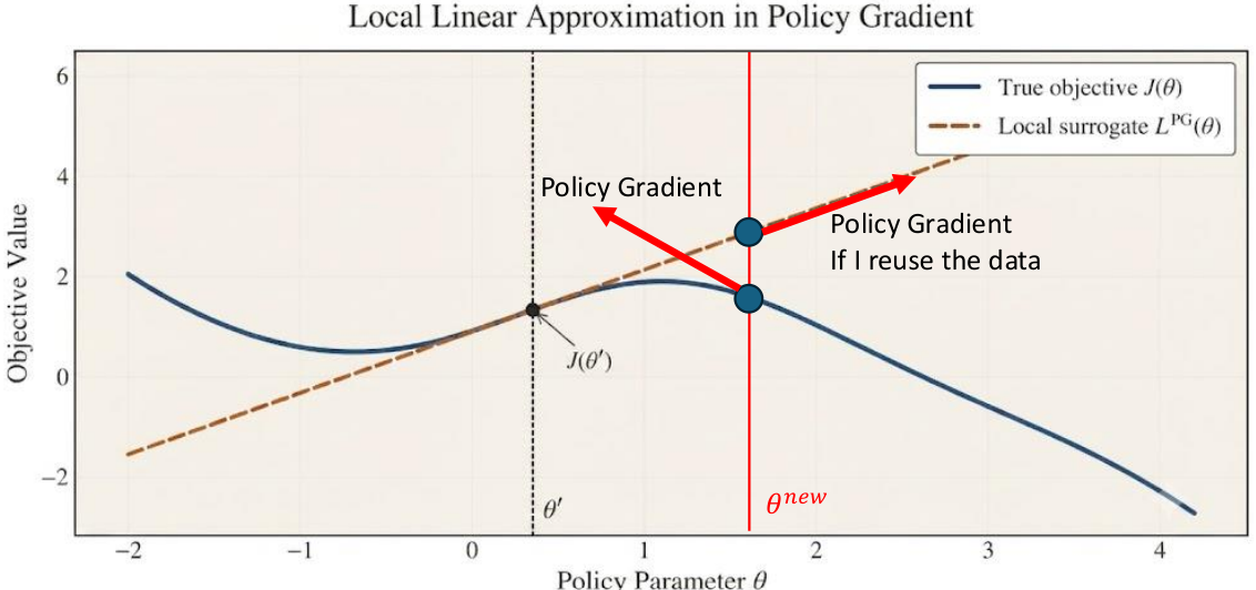
  • Multiple gradient steps with same data

Problem:

  • Data becomes off-policy

Idea:

  • Use Importance Sampling to estimate new gradient
Review: Desired Improvement in Off-Policy Steps

With J(\theta):=\mathbb{E}_{s_0}[V^\theta(s_0)]

We want this to be positive (minibatch epochs should improve objective):

J(\theta') - J(\theta) = \mathbb{E}_{\textcolor{red}{\tau\sim p_{\theta'}}}\Bigg[\sum_t A^\theta(s_t,a_t)\Bigg] =: \bar A(\theta')

Problem: Samples are with old policy \tau\sim p_{\theta}

In the last class, we got to this point:

J(\theta')-J(\theta)=\sum_{t=0}^{T-1}\mathbb{E}_{\textcolor{green}{s_t,a_t\sim p_\theta}}\Bigg[ \underbrace{ \frac{p_{\theta'}(s_t)}{p_{\theta}(s_t)} }_\text{State ratio} \cdot \underbrace{ \frac{\pi_{\theta'}(a_t|s_t)}{\pi_{\theta}(a_t|s_t)} }_{=: r_t(\theta')} A^\theta \Bigg]

Off-Policy Algorithm We Want

Process we want

  • Sample rollouts using \pi^\theta
  • Update \hat V estimate
  • Calculate advantage \hat A_t using GAE

K epochs of minibatch updates:

  • Find gradient of L(\theta') \approx \sum_{t=1}^H r_t \hat A_t
  • \theta' \leftarrow \theta' + \alpha\nabla_{\theta'}L(\theta')

Key modifications

  • Introduce a “loss surrogate” L(\theta') that uses samples from \pi_\theta
  • L drops the state ratio
  • The two agree to first order around \theta
  • Similar to A2C, but multiple learning epochs
Concerns
  1. Will this algorithm work?
  2. When can we ignore the distribution mismatch?

Recall: Biased Dice Example

Motivation

  • Roll 5 dice randomly
  • What is P(all 6’s)?

Importance sampling idea

  • Get a biased die that rolls 6 often
  • P(6) = 5/6, P(\lnot 6) = 1/6
  • Reweight samples by
w = \frac{(1/6)^5}{(5/6)^5} = 0.00032

Variance problem

  • What is P(all 1’s)?
  • Reweight samples by
w = \frac{(1/6)^5}{(1/30)^5} = 3125
  • Even a single 3125-weighted sample will dominate, other samples effectively get ignored
  • Effectively reducing dataset size
  • Increasing variance

Practical Challenge with Importance Sampling

Even ignoring the state ratio issue,

J(\theta') \approx \sum_{t=1}^H r_t A_t
  • Samples are collected once for several minibatch updates
  • A_t fixed for sampled actions

Will this work?

Problem

If we take many steps on the objective,

  • A_t > 0 --> r_t \uparrow ==> J \uparrow
  • A_t < 0 --> r_t \to 0 ==> term does not contribute to gradient
  • Terms with small r_t are effectively “ignored”
  • Effectively decreasing the effective dataset size, blowing up the sample variance

Root cause: we “trust” the sampled advantage too much

We will discuss how algorithms address this later today.

But first…

When Can We Ignore the State Ratio?

Importance Weight Factors

J(\theta')-J(\theta)=\sum_{t=0}^{T-1}\mathbb{E}_{{s_t,a_t\sim p_\theta}}\Bigg[ \textcolor{red}{ \underbrace{ \frac{p_{\theta'}(s_t)}{p_{\theta}(s_t)} }_\text{State ratio} } \cdot \underbrace{ \frac{\pi_{\theta'}(a_t|s_t)}{\pi_{\theta}(a_t|s_t)} }_{=: r_t(\theta')} A^\theta \Bigg]
  • Our samples are from the old policy \theta
  • New policy \theta' may not have visited the same states as \theta
  • State ratio: corrects for visiting different states under the new policy
  • Also called “distribution mismatch”

Problem: We cannot compute it directly – why?

  • p_{\theta'}(s_t) depends on the dynamics and on earlier actions under \theta'
  • We have no samples with \theta'!

Bounding Distribution Change: Deterministic Case, pt. 1

Claim: \pi_\theta close to \pi_{\theta'} ==> p_{\theta}(s_t) close to p_{\theta'}(s_t) ==> State ratio ~ 1

Proof:

What is \pi_{\theta}(a_t \neq \pi_\theta(s_t)) = ?

  • “\pi_\theta close to \pi_{\theta'}” -> assume \pi_{\theta'}(a_t \neq \pi_\theta(s_t)) \le \epsilon
  • Did \pi_{\theta'} make a “mistake” (different than \pi_\theta) in the first t steps?
  • If “no mistakes”, we end up at the same states as \pi_\theta would have:
    p_{\theta'}(s_t) = \underbrace{(1-\epsilon)^t}_\text{We made no mistakes} p_\theta(s_t) + (1 - (1-\epsilon)^t) p_\text{mistake}(s_t)

Based on Sergey Levine CS185 notes

Bounding Distribution Change: Deterministic Case, pt. 2

Claim: \pi_\theta close to \pi_{\theta'} ==> p_{\theta}(s_t) close to p_{\theta'}(s_t)

Proof (contd):

p_{\theta'}(s_t) = \underbrace{(1-\epsilon)^t}_\text{We made no mistakes} p_\theta(s_t) + (1 - (1-\epsilon)^t) p_\text{mistake}(s_t)
  • Subtract p_\theta(s_t) from both sides
p_{\theta'}(s_t) - p_\theta(s_t) = (1-(1-\epsilon)^t) \big(p_{\text{mistake}}(s_t) - p_\theta(s_t)\big)
  • Take absolute value and sum over s_t
  • \frac{1}{2}\sum_{s_t}\vert p_{\theta'}(s_t) - p_{\theta}(s_t)\vert
  • = (1 - (1-\epsilon)^t)\frac{1}{2}\sum_{s_t} \vert p_\text{mistake}(s_t) - p_{\theta}(s_t)\vert

Bounding Distribution Change: Deterministic Case, pt. 3

Claim: \pi_\theta close to \pi_{\theta'} ==> p_{\theta}(s_t) close to p_{\theta'}(s_t)

Proof (contd):

  • p_\theta are probability distributions, so \vert p_\text{mistake}(s_t) - p_{\theta}(s_t)\vert \le \vert p_\text{mistake}(s_t)\vert + \vert p_{\theta}(s_t)\vert \le 2
  • So we get

\le 1-(1-\epsilon)^t \le \epsilon t ~~ \blacksquare

  • This is Bernoulli’s inequality, but you can also approximately see (1-\epsilon)^t = 1 - \epsilon t + \mathcal O(\epsilon^2)

Proof caveat

  • Distance of p_{\theta}(s_t) to p_{\theta'}(s_t) is \sim \epsilon t
  • I.e. longer the horizon t, the worse the approximation
  • Limits horizon size in the replay buffer

Bounding Distribution Change: General Case

Claim: \pi_\theta close to \pi_{\theta'} ==> p_{\theta}(s_t) close to p_{\theta'}(s_t)

Sketch of proof:

Introduce a new metric: TVD = total variation distance

  • If \pi is discrete and finite -> \pi can be described as a vector -> TVD is half the \mathcal{L}_1-norm of the difference

“\pi_\theta close to \pi_{\theta'}”

  • ==> D_{\mathrm{TV}}(\pi_{\theta'}(\cdot \mid s_t), \pi_\theta(\cdot \mid s_t)) \le \epsilon ~~ \forall s_t
  • We use this shorthand: D_{\mathrm{TV}}(\pi_{\theta'}, \pi_\theta) \le \epsilon

We can prove that this means (not going to prove): P\big(\pi_{\theta'}(\cdot \mid s_t) \neq \pi_\theta(\cdot \mid s_t)\big) \le \epsilon.

Remember discrete case: \pi_{\theta'}(a_t \neq \pi_\theta(s_t)) \le \epsilon. Proof follows the same way.

Algorithm So Far: TVD

If D_{\mathrm{TV}}(p_{\theta}, p_{\theta'}) is small, we can show (not going to prove)

J(\theta') - J(\theta) \ge \sum_t \mathbb{E}[r_t A_t] - \sum_t 2 \epsilon_\mathrm{TV} t C
  • I.e. if you ignore the state ratio, the approximation error is bounded.
  • Bound C is based on the max horizon and reward terms

Let’s set

\theta' \leftarrow \arg\max_{\theta'} \; \mathbb{E}_{(s_t,a_t)\sim \pi_\theta}\left[r_t A^{\pi_\theta}(s_t,a_t)\right] \quad \text{s.t.} \quad D_{\mathrm{TV}}(\pi_\theta, \pi_{\theta'}) \le \epsilon_\mathrm{TV}
  • This ensures the first term in the preceding equation is positive (since \theta' = \theta gives 0)
  • Then J(\theta') - J(\theta) \ge -\text{small}(\epsilon_\mathrm{TV}) for small \epsilon_\mathrm{TV}.

Step back: \pi_\theta close to \pi_{\theta'} ==> Improvement in objective during minibatch epochs!

Proximal Policy Optimization (PPO)

PPO-Clip (Schulman et al., 2017)

Problem

  • TVD algorithm difficult to practically implement because of TVD constraint

PPO idea

  • No explicit distribution constraints
  • Add a heuristic to the objective

PPO Objective – Unclipped Term

L_\text{clip}(\theta) = \mathbb{E} \left[ \min \left( \textcolor{red}{r_t A_t}, \textcolor{blue}{\text{clip} \left( r_t, 1 - \epsilon, 1 + \epsilon \right) A_t} \right) \right], \quad r_t := \frac{\pi_{\theta'}(a_t)}{\pi_{\theta}(a_t)}

Unclipped objective: red

  • Weight r_t > 1 --> new policy assigns more probability to sampled action than old (data-collecting) policy
  • r_t < 1 --> getting less likely

Problem

  • Take a positively-advantaged action from the sample (A_t > 0)
  • In each minibatch epoch, r_t \uparrow ==> L \uparrow
  • Similarly for A_t < 0, r_t \to 0 ==> L \uparrow

A_t is not resampled for new policy, so minibatch epochs will keep pushing r_t

PPO Objective – Clipped Term

L_\text{clip}(\theta) = \mathbb{E} \left[ \min \left( \textcolor{red}{r_t A_t}, \textcolor{blue}{\text{clip} \left( r_t, 1 - \epsilon, 1 + \epsilon \right) A_t} \right) \right], \quad r_t := \frac{\pi_{\theta'}(a_t)}{\pi_{\theta}(a_t)}

Clipped objective: blue

  • Clip the ratio as a proxy for how far the policy has changed at a_t
  • E.g. \epsilon = 0.2 in (Schulman et al., 2017)
  • \theta'=\theta ==> no clipping
Question

What happens when ϵ is large?


Question

What happens when ϵ = 0?

PPO Objective – Combined

L_\text{clip}(\theta) = \mathbb{E} \left[ \min \left( \textcolor{red}{r_t A_t}, \textcolor{blue}{\text{clip} \left( r_t, 1 - \epsilon, 1 + \epsilon \right) A_t} \right) \right], \quad r_t := \frac{\pi_{\theta'}(a_t)}{\pi_{\theta}(a_t)}
  • Why do we take the minimum of the two terms?
  • Let’s work out some example cases.

Clipping Case: Positive Advantage

L_\text{clip}(\theta) = \mathbb{E} \left[ \min \left( \textcolor{red}{r_t A_t}, \textcolor{blue}{\text{clip} \left( r_t, 1 - \epsilon, 1 + \epsilon \right) A_t} \right) \right]
  • Sampled action was better than expected
  • Red term: r_t \uparrow ==> L \uparrow (increase probability of this “good” action)
  • After a couple of epochs, blue term becomes active (smaller than red term)
  • No further gain to L
  • \pi_{\theta'} = (1+\epsilon) \pi_\theta --> stop here
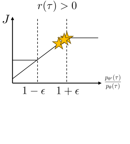
Image from Sergey Levine CS185 notes

Clipping Case: Negative Advantage, pt. 1

L_\text{clip}(\theta) = \mathbb{E} \left[ \min \left( \textcolor{red}{r_t A_t}, \textcolor{blue}{\text{clip} \left( r_t, 1 - \epsilon, 1 + \epsilon \right) A_t} \right) \right]
  • Sampled action was worse than expected
  • Red term: r_t \downarrow ==> L \uparrow (reduce probability of this “bad” action)
  • Clip toward the left (same as before)
Intuition

Don’t let a single advantage sample continually change the policy in its favor.
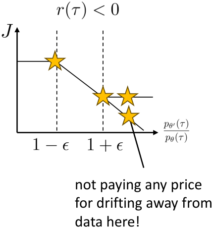
Image from Sergey Levine CS185 notes

Clipping Case: Negative Advantage, pt. 2

L_\text{clip}(\theta) = \mathbb{E} \left[ \min \left( \textcolor{red}{r_t A_t}, \textcolor{blue}{\text{clip} \left( r_t, 1 - \epsilon, 1 + \epsilon \right) A_t} \right) \right]

What if \theta' wants to go toward the right?

  • Action space can be high-dimensional
  • There is coupling between different dimensions
Question

Why do we not need to worry about the ratio “running away” in this case?

Image from Sergey Levine CS185 notes

What Happens During Minibatch Updates

L_\text{clip}(\theta) = \mathbb{E} \left[ \min \left( \textcolor{red}{r_t A_t}, \textcolor{blue}{\text{clip} \left( r_t, 1 - \epsilon, 1 + \epsilon \right) A_t} \right) \right]
  • Do rollout; get advantages A_t for actions
  • Over K epochs, r_t will get updated
Question

Will all ratios remain between 1−ϵ and 1+ϵ?


No, because of the reason from the previous slide

Image from Sergey Levine CS185 notes

Other PPO Tricks to Minimize Collapse

  • Implementations often stop the PPO epochs early if the measured divergence1 gets too large.
  • “Entropy regularization”: add \mathcal{H}(\pi_{\theta'}) to objective to prevent losing probability over actions
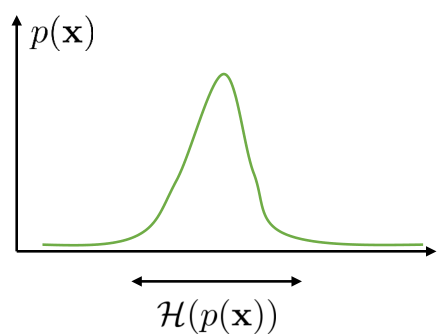
Image from Sergey Levine CS185 notes

1: TVD, or an approximation of it.

Summary: PPO Algorithm

Often implemented as Actor/Critic (estimate value function -> use for advantage)

  • Roll out the policy
  • Calculate advantage of samples using GAE as covered before: \hat A = \sum(\gamma\lambda)^{t'-t} \delta_{t'}

Minibatch epoch \theta' updates:

  • Compute objective gradient \hat g = \nabla_{\theta'} (L_{\mathrm{CLIP}}(\theta') \textcolor{gray}{+ \mathcal{H}(\pi_{\theta'})})
  • \theta' \leftarrow \theta' + \alpha \hat g

Where PPO is Useful

Chaotic or stochastic systems, where

  • small policy changes can have large effects;
  • larger step sizes can result in large policy changes.

Systems where data collection is moderately difficult1

  • Even with sim2real RL, complex dynamics can take time for physics simulation
  • PPO minibatch updates can make training faster
Examples
  • Robotics and locomotion – quadrupeds, humanoids
  • Game agents
  • Parallel environments sim2real RL – can parallelize data collection easily
1: Best sample efficiency is with off-policy methods

PPO Implementation Matters

Per (Engstrom et al., 2020), a lot of PPO’s success is due to “tricks” beyond the key paper ideas.

  1. Value function clipping: limit how far the critic moves from its old estimate each update
  2. Reward scaling: keep advantage and value targets at a consistent magnitude
  3. Reward clipping: clamp rewards to a fixed range (e.g. [-10, 10]) so rare outliers don’t dominate updates
  4. Observation normalization: standardize inputs so the network sees roughly unit-scale features
  5. Observation clipping: clamp normalized observations (e.g. to [-5, 5]) to prevent extreme inputs from causing spikes
  6. Gradient clipping: cap the gradient norm so a single bad batch can’t produce a huge parameter update

PPO Problem: Trust Region and Convergence

Does PPO actually constrain the divergence between old and new policies?


Small-sample issues

  • E.g. small sample size in replay buffer
  • Unsampled action probabilities could change without bound!

Non-monotonic improvement

Small \epsilon can also result in no improvement (gradient clipped to 0).

Failure example (Engstrom et al., 2020)

Let’s try to more systematically enforce the trust region.

KL Divergence & PPO-KL

KL Divergence

D_{\mathrm{KL}}(p || q) := \mathbb{E}_{x\sim p}[\log p(x) - \log q(x)]

Not symmetric!

  • Min D_{\mathrm{KL}}(p || q) ==> q high everywhere p high
  • Called “mode covering”

Can you see why?

  • Min D_{\mathrm{KL}}(q || p) ==> q low everywhere p is low
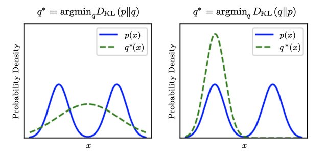
  • Fitting q^*(x) to target p(x)
  • Suppose q^* needs to be unimodal

Can you see the “mode covering”?

Example from (Goodfellow, 2016)

Quadratic Approximation

Taylor Series approximation of D_{\mathrm{KL}}(p_\theta || p_{\theta'}) when the two distributions are close

  • Say p_\theta and p_{\theta+\delta}
  • E.g. they are neural neworks parameterized by weights

Theorem:

D_{\mathrm{KL}}(p_\theta || p_{\theta + \delta}) = \tfrac{1}{2} \delta^T F(\theta) \delta

where F is the Fisher Information Metric

F(\theta) = \mathbb{E}_{x\sim p_\theta} (\nabla_\theta \log p_{\theta}(x)) (\nabla_\theta \log p_{\theta}(x))^T

Expected outer product of score vector \nabla_\theta \log p_{\theta}(x)

Forward vs. Reverse KL for PG

D_{\mathrm{KL}}(p_\theta || p_{\theta + \delta}) \approx \tfrac{1}{2} \delta^T F(\theta) \delta

  • Forward KL: D_{\mathrm{KL}}(\pi_\theta || \pi_{\theta'})
  • Reverse KL: D_{\mathrm{KL}}(\pi_{\theta'} || \pi_\theta)

Which should we use?

We want to use forward KL

  1. Quadratic approx F(\theta) is evaluated at the left argument --> want at \theta, where we collected samples
  2. Penalize new policy \pi_{\theta'} if it assigns low-probability to regions where \pi_\theta had probability --> prevent “collapse” or “ignoring actions”

Example from (Goodfellow, 2016)

Replacing TVD by KL Divergence

Pinsker’s Inequality: D_{\mathrm{TV}}(\pi_\theta, \pi_{\theta'}) \le \sqrt{\frac{1}{2} D_{\mathrm{KL}}(\pi_\theta || \pi_{\theta'})}

  • It is a lower bound, so D_{\mathrm{TV}} \le \epsilon <== D_{\mathrm{KL}} \le 2 \epsilon^2
  • In the algorithm, we can include a KL bound
  • Also, since \theta' = \theta + \alpha \hat g = \theta + \delta, the constraint becomes
    D_{\mathrm{KL}}(\pi_\theta || \pi_{\theta'}) = \frac{1}{2} \delta^T F(\theta) \delta \stackrel{?}{\le} 2 \epsilon^2

PPO-KL (Schulman et al., 2017): KL Penalty

L_{\mathrm{KL}}(\theta) = \mathbb{E}[r_t A_t] \textcolor{red}{- \beta D_{\mathrm{KL}}(\pi_\theta || \pi_{\theta'})}
  • Roll out the policy
  • Calculate advantage of samples using GAE as covered before: \hat A = \sum(\gamma\lambda)^{t'-t} \delta_{t'}

Minibatch epoch \theta' updates:

  • Compute objective gradient \hat g = \nabla_{\theta'} L_{\mathrm{KL}}(\theta')
  • \theta' \leftarrow \theta' + \alpha \hat g

Using average KL over batch:

  • \beta \leftarrow \max(0, \beta + \alpha_2(D_{\mathrm{KL}} - \epsilon)) <-- new

\beta update intuition

  • \epsilon is the KL “budget”
  • if KL changes more than that, we increase \beta
  • that results in a stronger KL penalty

PPO-KL was introduced in the same paper but has no clipping, and adds the KL penalty. PPO-Clip is the more common form.

Natural Policy Gradient (NPG)

Gradient Direction

Policy gradient vector: \theta' = \theta + \alpha \hat g

Notice that

  • A “small” \theta step can have a huge effect on \pi_\theta
  • To remain stable we would have to make \alpha small, and then convergence would suffer

Gradient purpose:

  • Policy gradient: Treat \theta as a Euclidean space, take a step in space of weights
  • Natural gradient: Don’t treat all \theta components uniformly
Natural Gradient: Motivating Example

Example of why it matters (Peters & Schaal, 2008):

  • policy: \pi_\theta(a|s) = \mathcal N(ks, \sigma^2), \theta = (k, \sigma)
  • reward: r(s_t, a_t) = -s_t^2 - a_t^2 (drive state and action to 0)
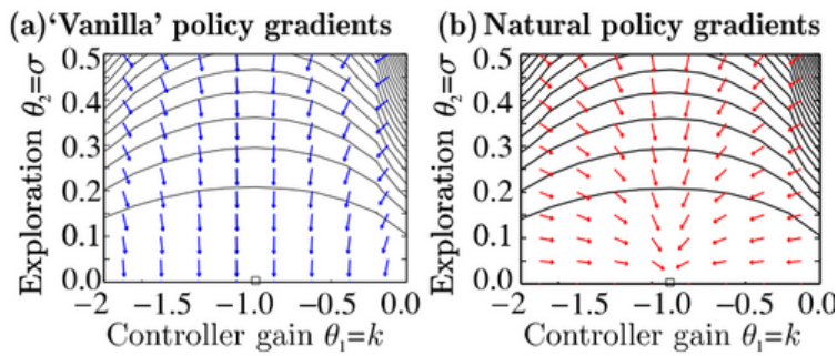
Blue arrows are vanilla gradients, red arrows are natural gradients; the square marks the optimum

Vanilla PG:

  • a step (\Delta k,\Delta \sigma) is mostly in \sigma
  • PG treats \theta components the same

What we want:

  • Equal-sized changes in \theta acknowledge that one affects mean and one affects variance
  • Natural PG measures the step by how much the policy changes (KL)
  • Update treats both directions fairly
  • Points more directly toward the optimum

Natural Gradient: Geometry Background

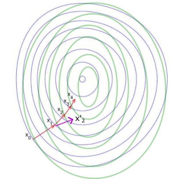
  • Gradient descent’s “steepest” direction depends on how we measure length
  • Not just “-\nabla L” in curved spaces
  • With metric M(x) associated with a point x: steepest direction maximizes decrease in L for fixed d^T M d
    • “Move 1 m within a disk, which direction is most downhill”
  • Solving gives d \propto -M^{-1}\nabla L
  • For distributions p_\theta, the metric is the Fisher matrix:
    F(\theta) = \mathbb{E}\left[\nabla\log p_\theta \, \nabla\log p_\theta^T\right]
    since \mathrm{KL}(p_\theta \| p_{\theta+\delta}) \approx \tfrac{1}{2} \delta^T F \delta
  • Natural gradient: F^{-1}\nabla L

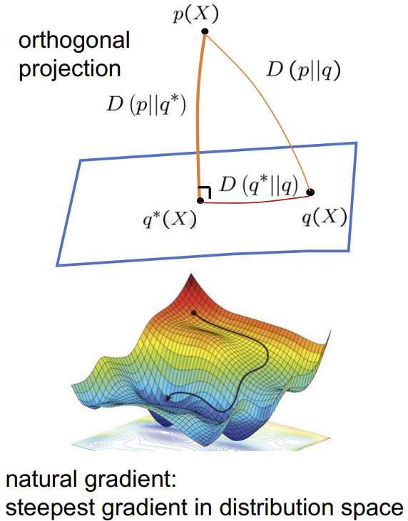
Image from https://noneq.c.u-tokyo.ac.jp/Stochastic_Thermodynamics_III/wp-content/uploads/2022/06/WOST-III_tutorial_oizumi.pdf

Algorithm So Far: NPG (Kakade, 2001)

  • Roll out \pi_\theta on N trajectories
  • Compute advantages with GAE: \hat A_t = \sum_{t'\ge t}(\gamma\lambda)^{t'-t}\delta_{t'}
  • Estimate at current \theta:
    • g = \mathbb{E}[\nabla_\theta\log\pi_\theta \hat A_t]
    • F = \mathbb{E}[\nabla_\theta\log\pi_\theta \nabla_\theta\log\pi_\theta^T]
  • Update: \theta \leftarrow \theta + \alpha F^{-1} g

Practical notes

  • Avoid forming or inverting F: solve Fx = g with conjugate gradient (Fisher-vector products)
  • (Kakade, 2001) uses a fixed step size; we can improve on this!

Trust-Region Policy Optimization (TRPO)

TRPO: KL Constraint, Constrained Step Size

So far

\theta \leftarrow \theta + \textcolor{red}{\alpha} F^{-1} g
  • NPG improves the gradient direction
  • Larger steps can still fail

How we can improve this

  • TRPO builds on NPG by adding a hard KL divergence constraint and a backtracking line search
  • Under the theory’s assumptions, this guarantees improvement of the policy.

TRPO: Constraint Version

  • Define a KL budget \epsilon_\mathrm{KL}
  • Step size allowed:
\Delta = \sqrt{\tfrac{2\epsilon_\mathrm{KL}}{g^T F^{-1} g}}\; F^{-1} g
  • Same direction as NPG
  • Step size found based on line search

TRPO Dual Descent Version (Slightly Faster)

  • Constrained problem: \max_{\theta'} \bar A(\theta') such that D_{\mathrm{KL}}(\pi_\theta \| \pi_{\theta'}) \le \epsilon_\mathrm{KL} (forward KL)

  • Make the inequality an equality, add it to the objective with multiplier \beta:

    \mathcal L(\theta', \beta) = \bar A(\theta') - \beta\,(D_{\mathrm{KL}}(\pi_\theta \| \pi_{\theta'}) - \epsilon_\mathrm{KL})

  • Dual gradient descent, alternating:

    • \theta' \leftarrow \arg\max_{\theta'} \mathcal L(\theta', \beta) (can stop after a few gradient steps)
    • \beta \leftarrow \beta + \alpha(D_{\mathrm{KL}} - \epsilon_\mathrm{KL})

How it works:

  • Constraint violated: \beta rises, so the KL penalty gets stronger
  • Constraint satisfied: \beta falls

Based on Sergey Levine CS185 notes

Intuition: TRPO Objective vs. NPG

NPG (fixed step): \theta' = \theta + \alpha F^{-1} g, where g = \nabla L

Penalized TRPO loss, using the quadratic KL:

L(\theta') - \beta\, D_{\mathrm{KL}}(\pi_\theta \| \pi_{\theta'}) \approx L(\theta') - \beta/2 (\theta' - \theta)^T F (\theta' - \theta)

Gradient w.r.t. \theta' (at \theta' \approx \theta):

\nabla_{\theta'}L = g - \beta F(\theta' - \theta)

Set \nabla_{\theta'}L = 0:

\theta' = \theta + \tfrac{1}{\beta} F^{-1} g

TRPO Monotonic Improvement Guarantee

(Schulman et al., 2015) show that

J(\pi')\ge L_\pi(\pi')-C
  • J is the expected return of the policy
  • L_\pi is the surrogate objective
  • C is related to the “max KL” (enforced by the KL budget)
Limitations
  • Only guaranteed to reach a local optimum (as with all gradient-based methods)
  • Assumes exact expectations while practical TRPO uses samples

Algorithm So Far: TRPO (Constraint Version)

  • Sample \{\tau^{(i)}\} from \pi_\theta, compute advantages \hat A_t with GAE
  • Gradient of surrogate at \theta: g = \nabla_{\theta'}\bar A(\theta')|_{\theta'=\theta}
  • Fisher matrix F (Hessian of forward KL D_{\mathrm{KL}}(\pi_\theta \| \pi_{\theta'}) at \theta)
  • Search direction: solve Fx = g with conjugate gradient (instead of F^{-1}g)
  • Full step: \Delta = \sqrt{\tfrac{2\epsilon_\mathrm{KL}}{x^T F x}}\, x, candidate \theta' = \theta + \Delta
  • Backtracking line search: shrink \Delta until the surrogate improves and D_{\mathrm{KL}}(\pi_\theta \| \pi_{\theta'}) \le \epsilon_\mathrm{KL}
  • \theta \leftarrow \theta'
TRPO practical problems, or why people use PPO
  • Computationally slower, but this isn’t the main reason
  • Slow convergence – line search can find very small step sizes

References

Engstrom, L., Ilyas, A., Santurkar, S., Tsipras, D., Janoos, F., et al. “Implementation matters in deep policy gradients: A case study on ppo and trpo.” arXiv preprint arXiv:2005.12729, 2020.
Goodfellow, I. “Deep learning.” MIT press, 2016.
Kakade, S. “A natural policy gradient.” Advances in neural information processing systems, 2001.
Peters, J., and Schaal, S. “Reinforcement learning of motor skills with policy gradients.” Neural networks, 2008.
Schulman, J., Levine, S., Abbeel, P., Jordan, M., and Moritz, P. “Trust region policy optimization.” International conference on machine learning, 2015.
Schulman, J., Wolski, F., Dhariwal, P., Radford, A., and Klimov, O. “Proximal policy optimization algorithms.” arXiv preprint arXiv:1707.06347, 2017.